Chapter 4 Results
4.1 Visual Pattern
In this chapter we will illustrate the result of the simulations. First we will start by showing some plots of different scenarios which in the estimations will be tested. The following graphs shows the scenario which the data of length 256 has been generated from a uniform distribution to make random grid is effectively non equally spaced and the curve \(f(x)=3x^3+4x^2\) is the function we want to estimate and the noise has been added to a signal-to-noise-ratio of 5. This curve has been chosen simply for demonstration purposes and we are primarily interested in estimating the function listed previously. Since this is a smooth function and the noise has been generated from a uniform distribution we expect that all the estimators could handle it well.
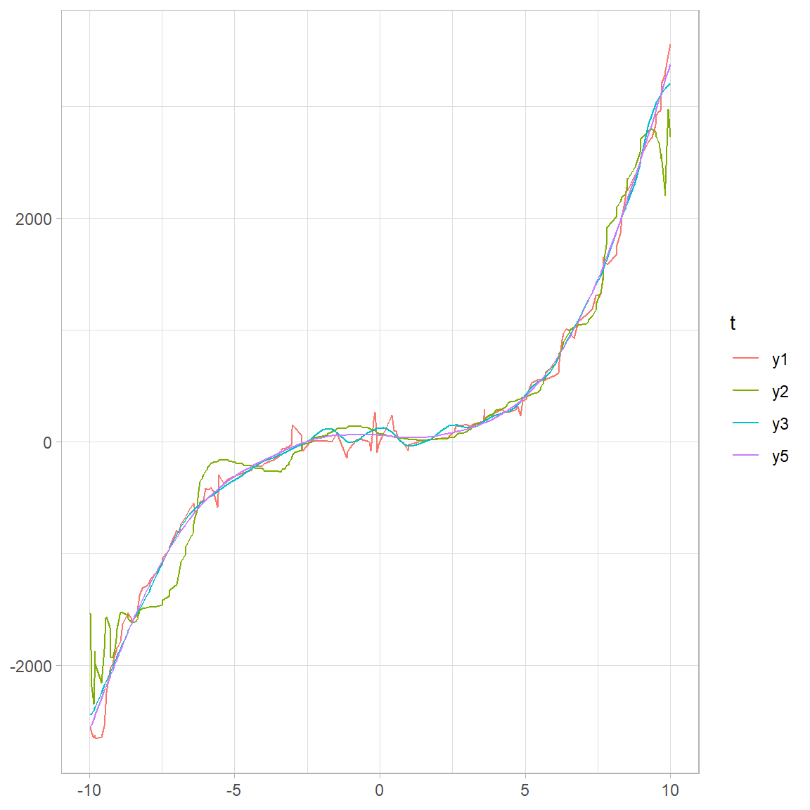
Figure 4.1: Estimate of the the curve \(f(x)=3x^3+4x^2\)
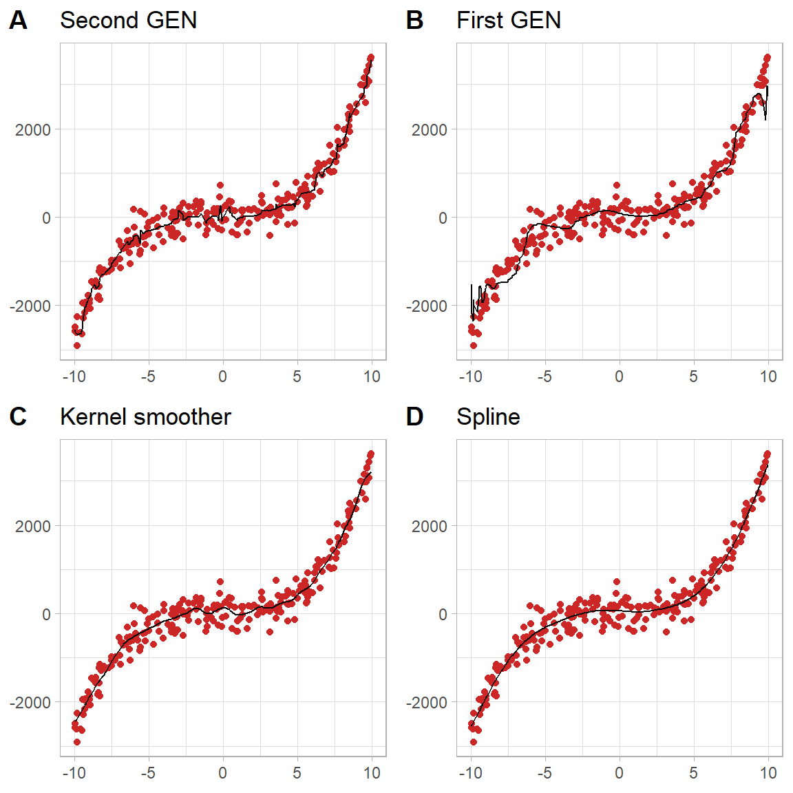
Figure 4.2: Estimate of the the curve \(f(x)=3x^3+4x^2\)
As expected, figure ?? show a good fit because there is not that much of variation in the data. Since the spline is less flexible than the other methods there is less variation in the spline estimated curve but obvious more biased and it is smoother. In the next graph we will move on to a more challenging curve to estimate. Just like the previous example the data has been sampled from uniform distribution with length 256 and the ratio for noise is the same. The curve that we are keen to estimate is the Doppler signal. We showed this signal in the previous section and it has the property of this has a considerable amount of variation close to zero and as we move away from zero the variation decreases. This property will make the estimation hard for the less flexible estimator. Moreover, non equally spaced nature in the data should cause the first generation Wavelet to struggle.
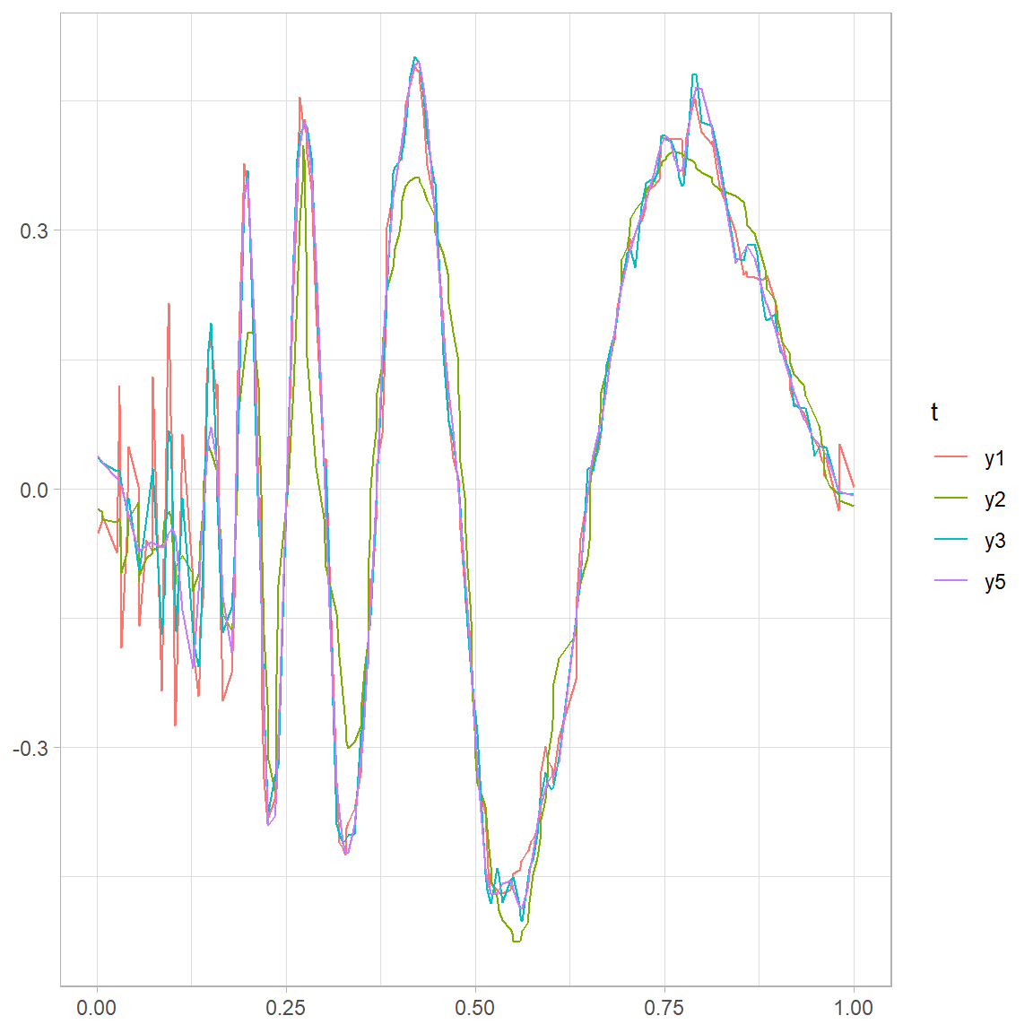
Figure 4.3: Estimates of Doppler signal on a uniforn grid
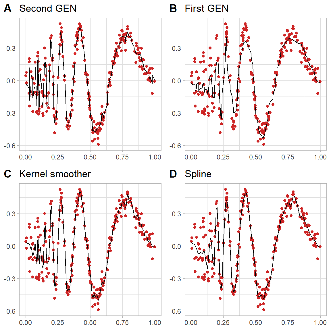
Figure 4.4: Estimates of Doppler signal on a uniforn grid
According to the graphs ?? spline estimator (D) could not capture the variation \(f\) when x is close to zero and it has avoided the peaks and it is biased. First generation Wavelet estimator(B) has explained some variation close to zero and it is similar to spline in the essence that struggles to capture the peaks in the data. In the next example the signal remains the same but the data will be generated from rigght-skewed to make it right-skewed. For this particular curve because the first half has more variation, having more data there will make it rather easier to estimate.
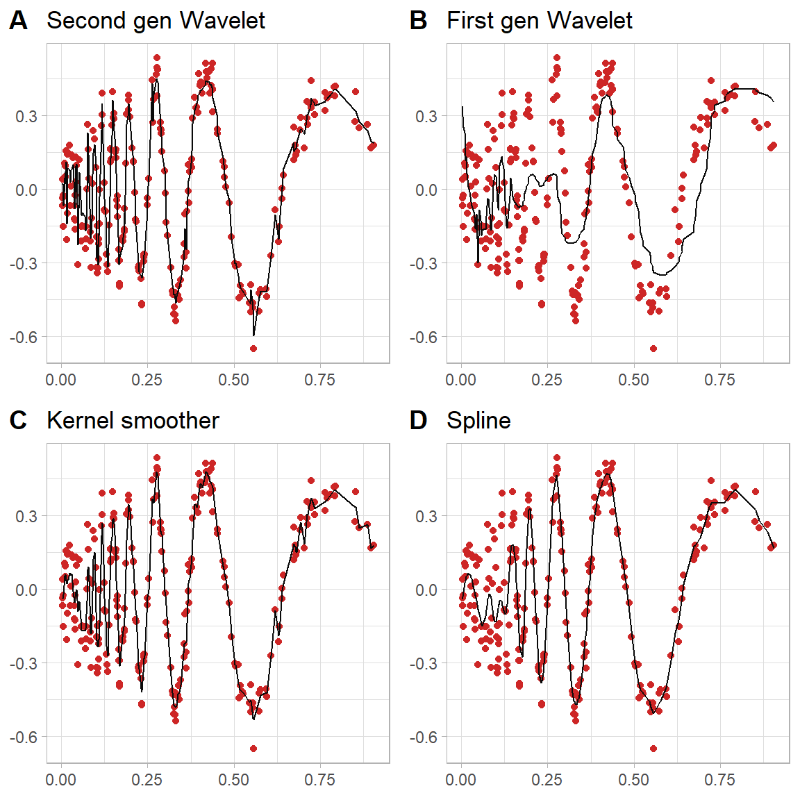
Figure 4.5: Estimate of Doppler signal on a right-skewewd grid
As expected the same trend has happened in the graph 4.5 second generation Wavelet(A) and Kernel smoother(C) estimators have done a good job but the other two are struggling. In next scenario we are going to generate the data from a left-skewed distribution and this means the first will have less data points close to zero. Therefore, we expect less flexible estimators to estimate the neighborhood around the zero.
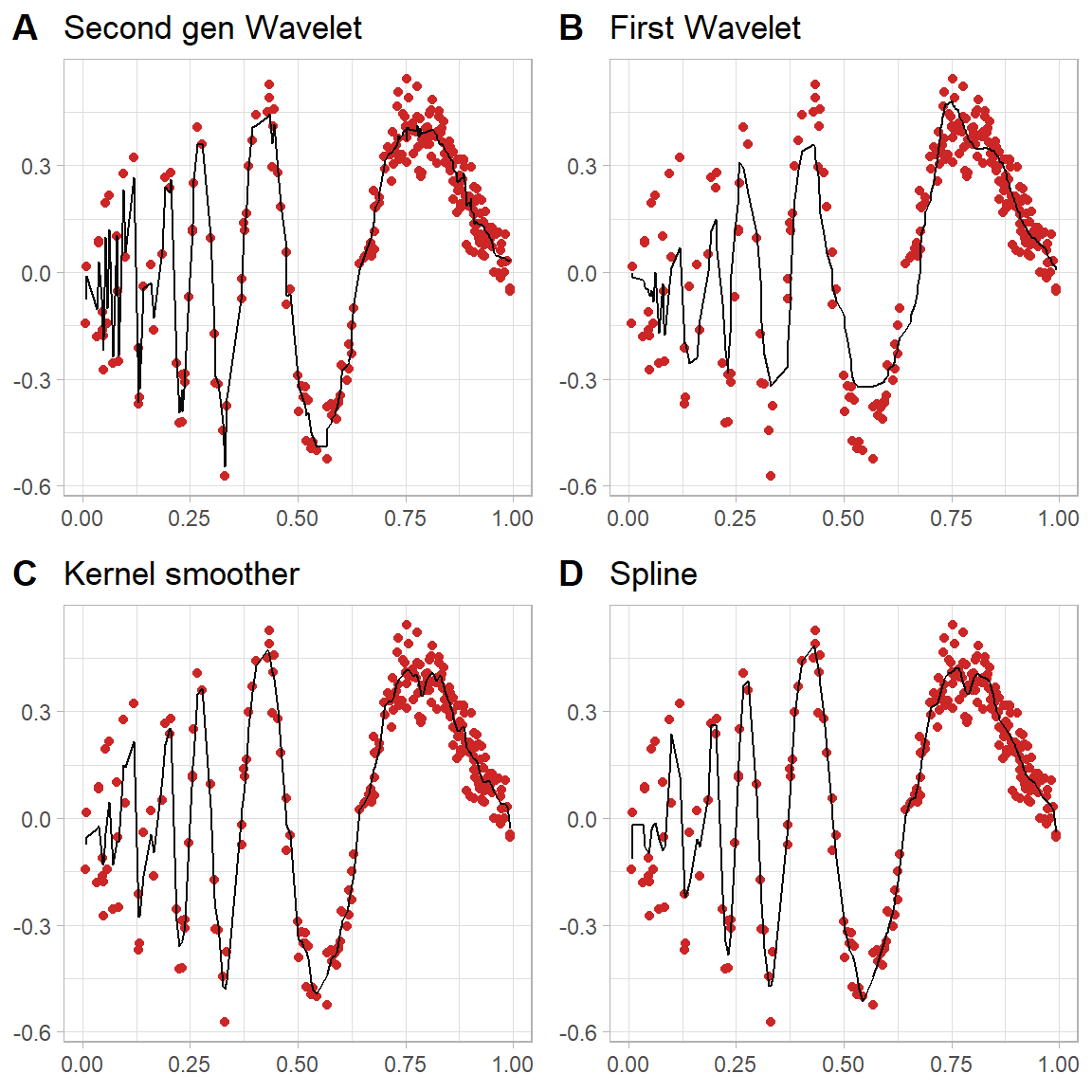
Figure 4.6: Estimates of a Doppler signal left-skewed grid
The figure 4.6 shows almost all estimators are biased near biased close to zero. The first generation has done worse and still far from being perfect it has avoided most of the peaks. The other three etimators have done a good job at capturing most of the variation and the peaks in the data. This result indicated as we mentioned before the second generation estimators is most of the time as good as other commonly used nonparametric estimators. However, we wish test this to simulated the data multiple time and calculated MSE and MAE to investigate this in a more precise way.
4.2 Basic functions
In this part we will present the results of simulation on some familiar functions including identity, quadratic, cubic, sine, cosine and exp. For this simulation data has been generated from \(\text{unif}(0,1)\) we will run the simulation for 50 time and the grid length will be 256. The signal-to-noise ratio has been kept 5 for this simulation. The results has been given below:
| estimators | Linear | Quad | Cubic | Sin |
|---|---|---|---|---|
| First GEN | 1.148 | 1.078 | 0.944 | 0.8078 |
| Second GEN | 0.8524 | 0.9862 | 0.7771 | 0.6987 |
| Kernel smoother | 0.8526 | 0.9864 | 0.7774 | 0.6988 |
| Spline | 0.8524 | 0.9862 | 0.7771 | 0.6987 |
| Cos | Exp |
|---|---|
| 0.2671 | 3.323 |
| 0.1898 | 2.411 |
| 0.1899 | 2.411 |
| 0.1898 | 2.411 |
| estimators | Linear | Quad | Cubic | Sin |
|---|---|---|---|---|
| First GEN | 13.67 | 13.15 | 12 | 11.76 |
| Second GEN | 11.86 | 12.64 | 10.46 | 10.84 |
| Kernel smoother | 11.86 | 12.64 | 10.47 | 10.84 |
| Spline | 11.86 | 12.64 | 10.46 | 10.84 |
| Cos | Exp |
|---|---|
| 6.597 | 23.13 |
| 5.671 | 20.43 |
| 5.671 | 20.43 |
| 5.671 | 20.43 |
The results in ?? and ?? shows under different conditions the second generation wavelet and kernel smoother and the spline can each be the best estimator based on MSE and MAE, whereas the first generation wavelet has a worse performance. The tables show that this pattern consstently. We continue with another table which represent the results for simulation on the list of signals the parameters and the generated grid is the same as above.
4.3 Signals
4.3.1 Uniform grid
| estimators | linchirp | mishmash | heavisine | doppler |
|---|---|---|---|---|
| First GEN | 151.7 | 389.9 | 141.9 | 14.73 |
| Second GEN | 10.38 | 221.1 | 90.6 | 1.554 |
| Kernel smoother | 13.9 | 220.4 | 90.79 | 1.782 |
| Spline | 18.59 | 288 | 94.53 | 2.654 |
| estimators | linchirp | mishmash | heavisine | doppler |
|---|---|---|---|---|
| First GEN | 158.6 | 256.6 | 156.8 | 45.31 |
| Second GEN | 34.56 | 184.5 | 126.2 | 15.05 |
| Kernel smoother | 39.44 | 179 | 126.3 | 15.93 |
| Spline | 46.96 | 219.8 | 128.2 | 18.09 |
The results in ?? and ?? show the first generation is not doing a performing well on the signal linchirp ,whereas the other three are relatively good. For the next signal mishmash the patterns gets repeated in both MSE and MAE the seconds generation very close to Kernel smoother. For the heavisine the same pattern gets repeated. At last, all the estimators seems to have better performance in performance to the first generation for the doppler signal both in MSE and MAE Now we will decrease the signal to noise ratio to 3 for the next simulation but all the parameter will be kept constant.
| estimators | linchirp | mishmash | heavisine | doppler |
|---|---|---|---|---|
| First GEN | 133.3 | 399.9 | 735.2 | 17.84 |
| Second GEN | 16.88 | 238.4 | 277.7 | 2.77 |
| Kernel smoother | 18.63 | 306.5 | 277.6 | 2.956 |
| Spline | 120.8 | 392.5 | 291.4 | 9.612 |
| estimators | linchirp | mishmash | heavisine | doppler |
|---|---|---|---|---|
| First GEN | 160 | 258.6 | 346.1 | 47.19 |
| Second GEN | 48.06 | 188.8 | 212.6 | 19.72 |
| Kernel smoother | 50.5 | 223 | 212.6 | 20.29 |
| Spline | 147.8 | 257 | 218.1 | 37.08 |
Tables ?? and ?? show that decreasing the signal-noise-ratio to three which effetively icraeses the variation has triggered an increasing pattern in both MSE and MAE. However, the relation between the performance of the estimators has remained the same. The second generation seems to be the estimator execpt for the heavisine in which Kernel smoother seems to be better. Now we will increase the signal to ratio to 6 but all the other parameter will be kept constant.
| estimators | linchirp | mishmash | heavisine | doppler |
|---|---|---|---|---|
| First GEN | 104.4 | 387 | 231.7 | 8.585 |
| Second GEN | 5.247 | 208.5 | 53.46 | 1.054 |
| Kernel smoother | 6.996 | 272.3 | 53.38 | 1.202 |
| Spline | 115.7 | 361.9 | 69.62 | 7.877 |
| estimators | linchirp | mishmash | heavisine | doppler |
|---|---|---|---|---|
| First GEN | 135.7 | 256.2 | 176.5 | 33.44 |
| Second GEN | 26.3 | 180.4 | 90.78 | 11.4 |
| Kernel smoother | 29.89 | 214.4 | 90.73 | 11.99 |
| Spline | 144 | 250 | 103.8 | 31.67 |
The above results in table ?? and ?? are every similar to the results of the noise ratio 5. Now we will move on with testing left-skewed grid in the next section.
4.3.2 Left skewed grid
| estimators | linchirp | mishmash | heavisine | doppler |
|---|---|---|---|---|
| First GEN | 123.5 | 382.6 | 1376 | 33.87 |
| Second GEN | 7.568 | 209.2 | 169.2 | 1.887 |
| Kernel smoother | 9.662 | 382.8 | 169.3 | 1.95 |
| Spline | 123.8 | 386.1 | 188.4 | 9.14 |
| estimators | linchirp | mishmash | heavisine | doppler |
|---|---|---|---|---|
| First GEN | 154.3 | 256 | 458.8 | 70.04 |
| Second GEN | 32.77 | 184.7 | 155.1 | 15.67 |
| Kernel smoother | 37.05 | 258.4 | 155.2 | 15.89 |
| Spline | 155.5 | 259.8 | 165.2 | 34.96 |
Based on results in table ?? and ?? on both MSE and MAE second generation wavelet estimator performs better than the first generation wavelet estimator. In addition, it seems the left skewed nature of the grid had a profound impact on accuracy of the other estimators too. Thereby, second generation wavelet estimator has beat all of them this time. Although, the kernel smoother is a very close in most of case for example the MAEs for example for heavisine. In the next part we will increase the signal-to-noise ratio to 5 to observe the changes.
| estimators | linchirp | mishmash | heavisine | doppler |
|---|---|---|---|---|
| First GEN | 144.9 | 383.2 | 2168 | 34.18 |
| Second GEN | 5.093 | 205.5 | 89.83 | 1.933 |
| Kernel smoother | 7.124 | 210.6 | 89.83 | 1.969 |
| Spline | 113.1 | 374.1 | 106 | 8.357 |
| estimators | linchirp | mishmash | heavisine | doppler |
|---|---|---|---|---|
| First GEN | 164.6 | 257.4 | 572.1 | 69.55 |
| Second GEN | 28.58 | 180 | 120 | 15.57 |
| Kernel smoother | 33.16 | 176.2 | 120 | 16.16 |
| Spline | 144.4 | 254.2 | 129.8 | 33.34 |
Increasing the signal to noise ratio from 4 to 5 has increased the MSEs and MAEs for the heavisine of first generation wavelet method sunbstantially according to tables ?? and ??. In contrast, both MSE and MAE for the other signals have not change significantly. Overall relations between different estimators is similar to the previous simulation except in the MAE table Kernel smoother is slighty better than second generation for mishmash and heavisine. Now will will increase the signal-to noise ratio to 6.
| estimators | linchirp | mishmash | heavisine | doppler |
|---|---|---|---|---|
| First GEN | 145.2 | 400 | 3330 | 34.53 |
| Second GEN | 6.858 | 185.8 | 65.09 | 1.099 |
| Kernel smoother | 9.211 | 186.3 | 65.12 | 1.22 |
| Spline | 119.2 | 353.9 | 84.77 | 8.068 |
| estimators | linchirp | mishmash | heavisine | doppler |
|---|---|---|---|---|
| First GEN | 163.1 | 259.2 | 735.4 | 73.14 |
| Second GEN | 31.41 | 171.4 | 103 | 12.32 |
| Kernel smoother | 35.66 | 164.9 | 103 | 12.79 |
| Spline | 146.5 | 246.3 | 117.1 | 31.99 |
The results in ?? and ?? does not shows that much of difference from the the signal-to-noise ratio 5. The overall relations remain the same between estimators. Comparing the results to the uniformly generating grid MSE and MAE of first generation estimators has gone up for all the signals. However, they are very close to the previous part for other estimators.
4.3.3 Right skewed grid
In this part the grid is chosen to be right-skewed. The below table shows the simulation using signal to noise ratio 4 and the other parameter remain constant.
| estimators | linchirp | mishmash | heavisine | doppler |
|---|---|---|---|---|
| First GEN | 136.5 | 447.1 | 3013 | 29.92 |
| Second GEN | 24.94 | 236 | 132.7 | 1.511 |
| Kernel smoother | 26.59 | 251.2 | 132.9 | 1.634 |
| Spline | 124.9 | 396.9 | 154.1 | 8.329 |
| estimators | linchirp | mishmash | heavisine | doppler |
|---|---|---|---|---|
| First GEN | 157.9 | 279.1 | 698.7 | 72.83 |
| Second GEN | 50.98 | 185.9 | 147.6 | 14.48 |
| Kernel smoother | 52.51 | 183.7 | 147.8 | 15 |
| Spline | 151.2 | 260.1 | 157.6 | 33.41 |
In the table ?? the results for second generation and Kernel smoother are close. In contrast, the estimates for first generation is substantially larger. The same pattern can be observed in the ??. Second generation wavelet method is the best except for the mishmash signal. In the following signal-to noise-ratio will be increase to 5.
| estimators | linchirp | mishmash | heavisine | doppler |
|---|---|---|---|---|
| First GEN | 144.9 | 442.7 | 1390 | 47.83 |
| Second GEN | 7.783 | 224.6 | 118.1 | 1.324 |
| Kernel smoother | 9.761 | 271.3 | 118.2 | 1.561 |
| Spline | 113.6 | 367.5 | 132.2 | 8.326 |
| estimators | linchirp | mishmash | heavisine | doppler |
|---|---|---|---|---|
| First GEN | 158 | 268.1 | 475.3 | 89.54 |
| Second GEN | 28.57 | 184.6 | 113.7 | 12.58 |
| Kernel smoother | 33.07 | 210.9 | 113.8 | 13.38 |
| Spline | 143.9 | 248.1 | 125.4 | 32 |
According to table ?? and ?? change in signal-to-noise-ratio does not change the estimates substantially; however, the estimates of the heavisine seems to decrease both in ?? and ??. In the following able the signal-to-noise-ratio will be increased to 6.
| estimators | linchirp | mishmash | heavisine | doppler |
|---|---|---|---|---|
| First GEN | 1.91 | 1.642 | 2.502 | 1.711 |
| Second GEN | 0.7898 | 0.5211 | 0.4299 | 0.4406 |
| Kernel smoother | 0.7898 | 0.5216 | 0.4299 | 0.4407 |
| Spline | 0.7898 | 0.5211 | 0.4299 | 0.4406 |
| estimators | linchirp | mishmash | heavisine | doppler |
|---|---|---|---|---|
| First GEN | 18.46 | 17.23 | 21.12 | 17.93 |
| Second GEN | 10.87 | 9.334 | 8.195 | 8.89 |
| Kernel smoother | 10.87 | 9.337 | 8.195 | 8.889 |
| Spline | 10.87 | 9.334 | 8.195 | 8.89 |
For this analysis the results in both ?? and ?? are substantialy smaller than the previoous part, it seems that the signal-to-noise-ratio noticeably effect the estimates and pushed them down.