Chapter 3 Methodology

3.1 Simulation

In this project we want to test our estimators on a signal whose function has been constructed on a non equally-spaced grid. The ultimate goal is to calculate the mean square error and mean absolute error associated which each estimator. This will give us a relative measure to compare the estimators and their strengths and weaknesses plus the possible conditions that will force them to fail to address the variation in the data correctly. To generate such data first we will obtain a random sample of size n from a probability distribution. First, we will use \(X \sim \text{unif}(0,1)\) which will provide us with a grid which is not skewed to either left or right. Then we will plug in this data in a function such as Quadratic function, Cubic function, Sinusoidal function, Cosinusoid function to derive the \(Ys\). \[ f_1(x)=x,\quad \text{Linear}\] \[f_2(x)=x^2,\quad \text{Quadratic}\] \[f_3(x)=x^3,\quad \text{Cubic}\] \[f_4(x)=sin(x),\quad \text{Sinusoid}\] \[f_5(x)=cos(x),\quad \text{Cosinusoid} \]

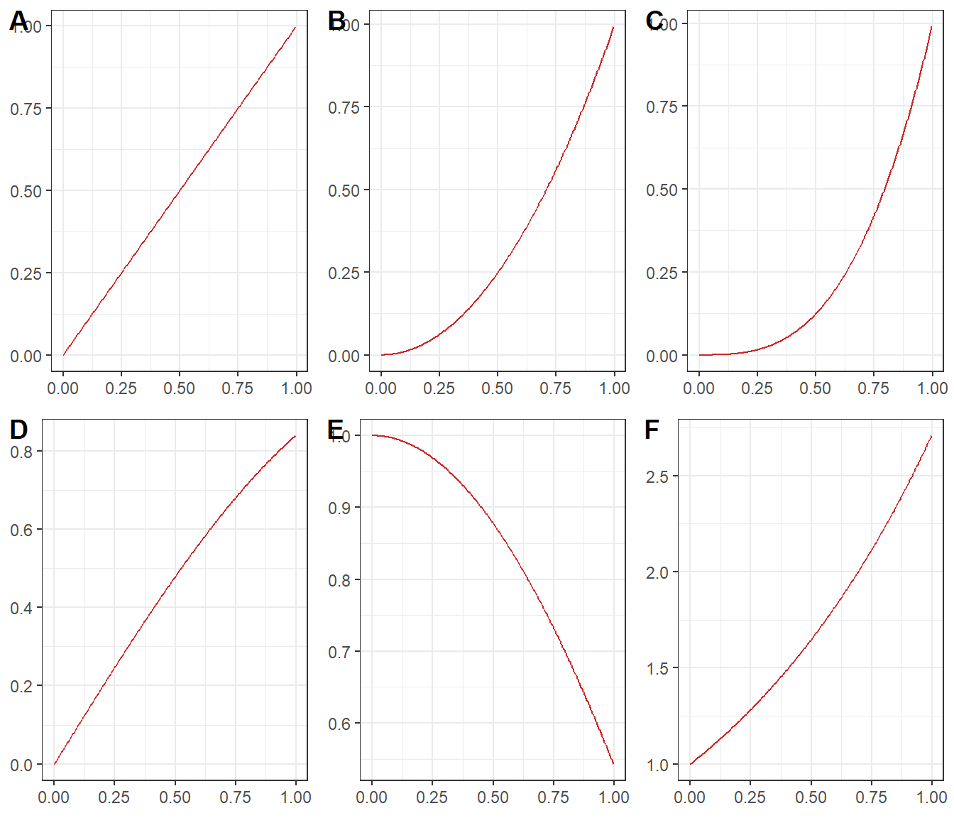
Figure 3.1: Plot of Basic functions analysed in this project

In the figure ?? A is the Linear function, B is the Quadratic function, C is the Cubic function, D is sinusoidal function, E is cosinusoidal function and F is Exponential function. In addition to these basic functions the generated grid will be used to generate signals such as linchirp, Doppler, heavisine and the Mishmash. Definition of these signals is not simple; therefore, the plot of these signals has been provided in figure 3.3.

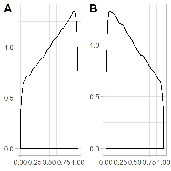
Back to our simulation, after generating the grid from \(X \sim \text{unif}(0,1)\) the same procedure will be carried out for the data generated from a left skewed mixture of \(\text{beta}(2,1)\) and \(\text{unif}(0,1)\). And for the right skewed mixture of \(\text{beta}(1,2)\) and \(\text{unif}(0,1)\). These distributions have been generated using the regularized beta incomplete beta function from the zipFR package(Evert & Baroni, 2007). The density plot of these distribution has been provided below:

Figure 3.2: Density plot of Left and Right skewed distrtibution used for generating grid

We have chosen these distribtions to make sure the generated grid point do start close to zero in a left-skewed case and do finish near one in the rightskewed case. In other words we wanted to have a grid which contain point from the entire \((0,1)\) interval and this is important because the true value \(f\) that we want to compare our estimates \(\hat f\) which is constructed from the previously mentioned functions and the equally spaced grid which starts from zero and goes all the way through one. It is important to try both left and right skewed grids and the reason for this is the non symmetric shape of signals. For instance, Doppler signals are more dense in the left hand side close to zero, so if the sample contains a small number of point on the right hand side it is not hard to see why some estimators will struggle to came up with a good estimate.

The signals in this project have been generate using the make.signal2 in the CNLTreg (Nunes & Knight, 2018) package in R which is a modified version of make.signal in S-plus and has the ability to generate signals on an specified grid. In addition, the plot in this project has been created using the ggplot2 package (Wickham, 2016) and the cowplot(Wilke, 2019) has used to put the ggplot generated plots into a panel.

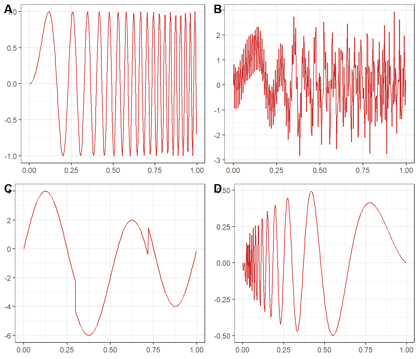
Figure 3.3: Plot of signals analysed in this project

In figure 3.3 A is Lincharp, B is Mishmash, C is Heavisine and D is Doppler. Moreover, noise will be generated from a normal distribution with zero mean and a variance signal-to-noise ratio and will be added to the data. We will change the signal-to-noise ratio to observe the behavior of the estimators see (3.2). The estimated values from the estimators will be recorded.

In this project four different estimators have been used to estimate the regression function. First, for first generation wavelet the functions from wavethresh package. First we use the function wd which performs the wavelet discrete transform and then use threshold function drop the coefficent below the threshold and then we use function wr to perform the reverse wavelet trtansform. For these functions the parameters where kept as default. Second, for the second generation wavelet the regression function from the CNLTreg package (Nunes & Knight, 2018) has been used. This function gets takes the signal and grid value as argument returns the estimates. Parameter P in this function is the number of times that the algorithm gets applied to the data then it averages obtained estimates to obtain the final estimates. Moreover, selecting a P larger than 2 is computationally intensive and according to our tests, in our does not significantly improve the MSE, thus, we use P=2. Third, for kernel smoothing regression np package (Hayfield & Racine, 2008) has been used, this package contains all kind of nonparametric methods. The regression type for the np is chosen to be local constant and the bandwidth selection has been done by Kullback-leibler cross-validation(Hurvich, Simonoff, & Tsai, 1998). Fourth, for spline the mgcv package was used (Wood, 2003). This package has different functions built in to it including spline smoothing and generalized additive models. In this project to choose the optimal number of knots for penalized B-splines we have used the function gam.check which is provided in the package. The optimal K was 60 for all the signals. This is because the number of knots should be large enough to avoid underfitting. However, if the number of knots is more than enough it would avoid overfitting by penalizing term in equation (2.4).

3.2 Calculating MSE

Our purpose is to estimate the estimate \(f\) in equation below: \[\begin{equation} Y_{ij}=f(t_j)+\epsilon_{ij},\quad \epsilon\sim N(0,\sigma^2) \tag{3.1} \end{equation}\] In (3.1) we know that \(f(t)\) which is the true value of the function of interest. We obtain it by pluging an equally space grid with desirable amount of time points in the function. Furthermore, \(\sigma\) is calibrated by the following equation with respect to signal-to-noise-ratio \(r\): \[\begin{equation} \sigma^2=\frac{Var(f(t_i))}{r},\quad i=1,\dots,M \tag{3.2} \end{equation}\] Where \(t_i\) is a fixed grid of lenght \(M\), therefore \(f(t_i)\) is a vector of lenght \(M\) and we calculate the variance of it. In each iteration we calculate the estimate for each time point and record it. Therefore, after N iterations we have \(N\) estimate of length \(M\) for the signal of interest. We have to note that for the estimators that take the unequal-spaced grid as an argument we have to interpolate the estimated value to a equal-space grid. This will allow us to compare different estimators by calculating the MSE. Now we will discus how to calculate MSE. The below formula will be used to calculate the MSE: \[ \begin{aligned} MSE=\mathbb{E}(\hat f,f)(t)&=\mathbb{E}(\hat f(t)-f(t))^2\\ &=\mathbb{E}[\hat f(t)-\mathbb{E}(\hat f(t))]+\mathbb{E}[\hat f(t))-f(t)]^2\\ &=\mathbb{E}[\hat f(t)-\mathbb{E}(\hat f(t))]^2+\mathbb{E}[Bias(\hat f(t),f(t))]^2\\ &=Var(\hat f(t))+Bias^2(\hat f(t),f(t))\\ \end{aligned} \] In the above formula \(f(t)\) is the true value of the function or signal \(f\) at point \(t\) which we wish to estimate. To obtain true value first we generate a equally space grid which is effectively a sequence of numbers with constant increment. Then we plug it in to our function and now we have the true values for each time \(t\). On the other hand, \(\hat f(t)\) is a the estimate that we get from our estimator. Using the same values we also use the following formula to calculate the Mean absolute error: \[MAE=\mathbb{E}(|\hat f(t)- f(t)|)\]. We will use MAE because it is considered to be an alternative for MSE(Friedman, Hastie, & Tibshirani, 2001). As mentioned above after recording the estimates with length of M since the grid is of length \(M\) therefore the estimates would have the same length and associated interpolated values would have the same length too. Since we are repeated the procedure for N time we will end up with a dataset of interpolated estimated values which is a \(M\times N\) matrix. Although we mentioned interpolation is not good practice, we do it only for purpose of calculating the MSE and MAE. To calculate the bias of the estimates at point \(t\) we will take the average of the each row of the data set and subtract it from the true value of the regression function on that point. We calculate the variance of estimator at each point by simply calculating variance of each row of the data. Then we can calculate MSE by the this formula \(MSE=Bias^2+Var\). Then we can calculate \(MSIE\) by calculating the mean of \(MSE\) of all points.